The PCA Trick I Use All the Time (But Almost No One Talks About)

A complete hands-on tutorial (with code) using volatility features to create one clean, interpretable signal for your trading models.

You’ve probably used PCA before.
Maybe to reduce dimensionality, maybe just because “it’s what everyone does.”

But here’s the thing: most people use it wrong — especially in trading.

In this newsletter, I’ll show you the exact trick I use to turn 12 noisy volatility features into one clean, powerful signal.
No black box. No information loss. Just feature engineering.

Let’s dive in.

1. What Most Traders Get Wrong About PCA?

Applying PCA on your entire feature set might sound like a smart move.
It reduces dimensionality, removes multicollinearity… what's not to like?

But here’s the catch:
➡️ You lose interpretability.
➡️ You don’t know what your new features really contain.
➡️ Tools like SHAP or feature importance become meaningless, because you’re working with abstract linear combinations of everything.

PCA turns your input into a black box.
And in trading, that’s rarely a good idea.

2. How to Keep Interpretability When Using PCA

Instead of applying PCA globally, I use it selectively — on feature groups that measure the same thing.

• Apply PCA on volatility features → get one clean volatility variable

• Apply PCA on trend features → get one synthetic trend signal

• Apply PCA on regime indicators → compress into one regime score

This way, I reduce dimensionality without losing interpretability, and my model stays transparent and clean.

Let me show you how that works in practice, using volatility features.

3. What Is PCA (and Why It Matters in Trading)

PCA (Principal Component Analysis) helps reduce redundancy by turning correlated features into uncorrelated components. It’s especially useful when you have dozens of overlapping signals (like volatility or trend indicators).

But markets aren’t linear. That’s why I often prefer Kernel PCA, which captures more complex, non-linear patterns.

✅ Simplifies your feature space
✅ Keeps essential structure
✅ Works better when signals interact in unpredictable ways

4. Step-by-Step: How to Build a Synthetic Volatility Feature

Now that we’ve seen the theory, let’s put it into action.
In the next steps, we’ll go through the full process. From raw OHLCV data to a clean, synthetic volatility feature, using Kernel PCA.

4.1. Data Import & Feature Engineering

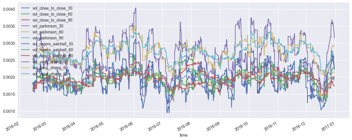
Let’s start by importing our dataset and creating a set of volatility-related features.
We’ll use four estimators — each calculated over 3 rolling windows — for a total of 12 volatility features.

# Import the dataset
from quantreo.datasets import load_generated_ohlcv
df = load_generated_ohlcv().loc["2016"]  # Focus on one year for clarity

Now let’s create our volatility features using Quantreo’s built-in functions:

import quantreo.features_engineering as fe

# Standard volatility
df["vol_close_to_close_30"] = fe.volatility.close_to_close_volatility(df, window_size=30)
df["vol_close_to_close_60"] = fe.volatility.close_to_close_volatility(df, window_size=60)
df["vol_close_to_close_90"] = fe.volatility.close_to_close_volatility(df, window_size=90)

# Parkinson volatility
df["vol_parkinson_30"] = fe.volatility.parkinson_volatility(df, window_size=30)
df["vol_parkinson_60"] = fe.volatility.parkinson_volatility(df, window_size=60)
df["vol_parkinson_90"] = fe.volatility.parkinson_volatility(df, window_size=90)

# Rogers-Satchell volatility
df["vol_rogers_satchell_30"] = fe.volatility.rogers_satchell_volatility(df, window_size=30)
df["vol_rogers_satchell_60"] = fe.volatility.rogers_satchell_volatility(df, window_size=60)
df["vol_rogers_satchell_90"] = fe.volatility.rogers_satchell_volatility(df, window_size=90)

# Yang-Zhang volatility
df["vol_yang_zhang_30"] = fe.volatility.yang_zhang_volatility(df, window_size=30)
df["vol_yang_zhang_60"] = fe.volatility.yang_zhang_volatility(df, window_size=60)
df["vol_yang_zhang_90"] = fe.volatility.yang_zhang_volatility(df, window_size=90)

At this stage, you have a full set of volatility features — but they’re highly correlated with each other. To move forward, you need a way to retain as much information as possible while using as few variables as necessary.

4.2. Split, Standardize & Apply Kernel PCA

Before applying PCA, we split the dataset chronologically (no shuffling!) and standardize the volatility features.

from sklearn.preprocessing import StandardScaler
from sklearn.decomposition import KernelPCA

# Split the data chronologically (80% train, 20% test)
train_size = int(len(df) * 0.8)
train_df = df.iloc[:train_size].copy()
test_df = df.iloc[train_size:].copy()

Now we scale the features — important for PCA, especially Kernel PCA which is geometry-based.

scaler = StandardScaler()
scaler.fit(train_df[vol_features])  # Fit only on training set

# Scale both datasets using the same scaler
train_df_scaled = scaler.transform(train_df[vol_features])
df_vol_scaled = scaler.transform(df[vol_features])

We apply Kernel PCA to reduce our 12 volatility features into a single synthetic component.

# Apply Kernel PCA
pca = KernelPCA(n_components=1)
pca.fit(train_df_scaled)  # Fit on train set

# Transform the entire dataset
import pandas as pd
df["volatility"] = pca.transform(df_vol_scaled)

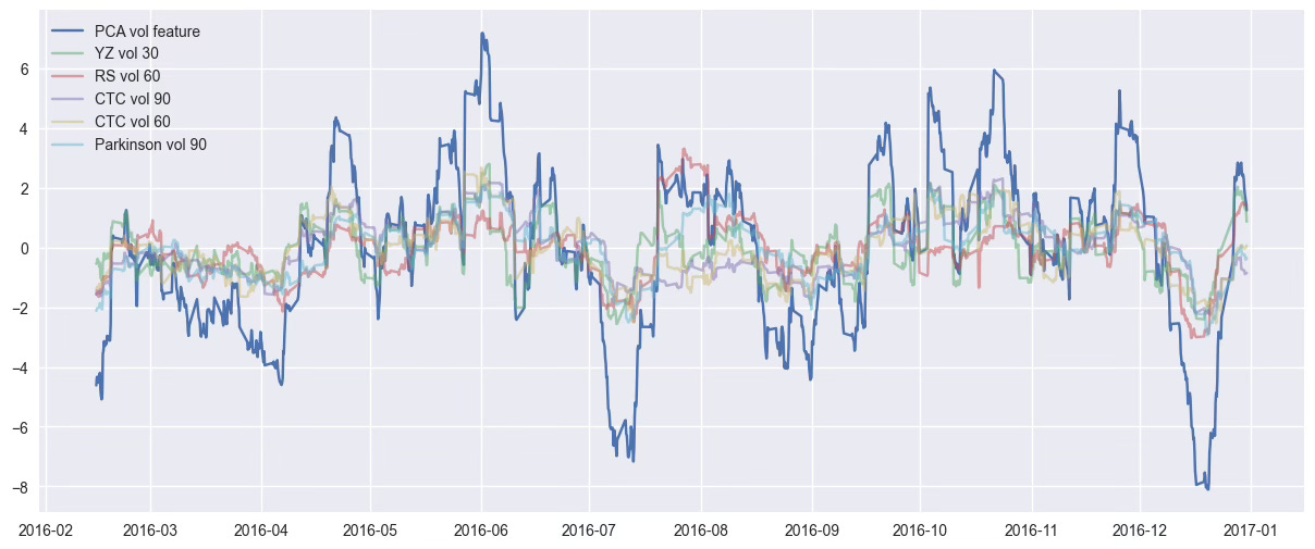
4.3. Visualize & Compare the Result

Let’s visualize the new volatility feature compared to a few original indicators.
We should see that it captures the same market dynamics in a cleaner, more compact way.

import matplotlib.pyplot as plt
plt.style.use("seaborn-v0_8")
plt.figure(figsize=(15, 6))

plt.plot(df["volatility"], label="PCA vol feature")
plt.plot(df_vol_scaled[:, vol_features.index("vol_yang_zhang_30")], label="YZ vol 30", alpha=0.5)
plt.plot(df_vol_scaled[:, vol_features.index("vol_parkinson_90")], label="Parkinson vol 90", alpha=0.5)
plt.plot(df_vol_scaled[:, vol_features.index("vol_close_to_close_60")], label="CTC vol 60", alpha=0.5)

plt.legend()
plt.title("Synthetic Volatility Feature vs Original Indicators")
plt.show()

This new feature is now ready to be used in any downstream model or strategy —
with less noise, no redundancy, and no black box effect. 🔥

💻 Want to take a look to the code? Click here.

By applying PCA selectively on volatility features, we’ve created a single, synthetic signal that captures the essential market dynamics — without the noise or redundancy of using all 12 raw indicators.

This approach:

• Keeps your model clean and interpretable

• Reduces overfitting risks

• Preserves the core information in fewer dimensions

🧠 Use it as a smart input in your trading models, or as a standalone volatility regime filter.
And remember: small tricks like this can make a big difference.