KAMA Explained Like Never Before

Understand its logic. Master its formula. Use it better than 99% of traders.

Apr 18, 2025

Everyone talks about SMA, EMA, even WMA.
But the one moving average that adapts to market conditions in real time?
Almost no one understands it, let alone uses it properly.

In this issue, we break down Kaufman’s Adaptive Moving Average (KAMA) like never before.
Formulas, mechanics, strengths, flaws… Everything you need to actually master it.

If you want to stop overreacting to noise and start tracking real trend shifts,
KAMA might just become your new favorite tool.

1. The Origin of KAMA

Kaufman’s Adaptive Moving Average (KAMA) was introduced by Perry J. Kaufman in the 1990s, in his book Smarter Trading.

Unlike most moving averages, KAMA wasn’t designed to smooth price just for the sake of clarity. It was built to adapt.

Kaufman observed that markets constantly alternate between noise and trend. Traditional averages either lag too much or react too wildly. His goal:
Create a moving average that stays flat in sideways markets and quickly follows price during real momentum.

The result is a dynamic filter that adjusts its sensitivity based on market efficiency. And it still holds up today.

2. How KAMA Really Works?

KAMA adapts to market conditions by adjusting its smoothing based on how efficient the price movement is.
It’s calculated in three steps.

2.1. Efficiency Ratio (ER)

The Efficiency Ratio measures how directional the price movement is over a given period. It tells us how "clean" the price movement has been over a given window.

If price moves straight up, ER is close to 1. If it oscillates back and forth, ER drops toward 0.

\(ER_t = \frac{|\text{Price}_t - \text{Price}_{t - l1}|}{\sum_{i=t - l1 + 1}^{t} |\text{Price}_i - \text{Price}_{i - 1}|} \)

Numerator: net change over the period
Denominator: total movement (sum of all price changes)
l1: efficiency lookback (typically between 10 and 30)

⚠️ Note: You can absolutely use l1 values greater than 30, especially for long-term strategies. Just keep in mind that increasing l1 reduces noise but also adds more lag.
It's all about the trade-off. Pick the right balance based on your timeframe and how reactive your strategy needs to be.

2.2. Smoothing Constant (SC)

This is the adaptive weight applied to the price, based on ER.

First, compute the constants for the fastest and slowest EMAs:

\(SC_{\text{fast}} = \frac{2}{l2 + 1}, \quad SC_{\text{slow}} = \frac{2}{l3 + 1} \)

Then blend them using ER:

\(SC_t = \left[ ER_t \cdot (SC_{\text{fast}} - SC_{\text{slow}}) + SC_{\text{slow}} \right]^2 \)

l2 = fast length (e.g. 2) (called also fast EMA period even if we do not compute an EMA)
l3 = slow length (e.g. 30) (called also slow EMA period even if we do not compute an EMA)

2.3. Recursive Calculation of KAMA

Like any EMA, KAMA is updated step by step:

\(KAMA_t = KAMA_{t - 1} + SC_t \cdot (Price_t - KAMA_{t - 1}) \)

This formula ensures:

In low efficiency (range), SC is small → KAMA barely moves
In high efficiency (trend), SC is large → KAMA reacts faster

3. Step-by-Step KAMA Calculation in Python

Let’s break down the full KAMA calculation into clear, isolated steps.

We’ll go from a raw price series to the final smoothed output, in three phases:

3.1. Compute Efficiency Ratio (ER)

The first step is to calculate how directional the price movement is over the last l1 periods.

def compute_er(price: np.ndarray, l1: int) -> np.ndarray:
    er = np.full_like(price, fill_value=np.nan, dtype=float)

    for t in range(l1, len(price)):
        change = abs(price[t] - price[t - l1])
        volatility = np.sum(np.abs(price[t - l1 + 1:t + 1] - price[t - l1:t]))
        er[t] = change / volatility if volatility != 0 else 0

    return er

3.2. Compute Adaptive Smoothing Constant (SC)

Using the ER, we calculate a smoothing constant that adapts between a fast and slow EMA.

def compute_sc(er: np.ndarray, l2: int, l3: int) -> np.ndarray:
    sc = np.full_like(er, fill_value=np.nan)

    sc_fast = 2 / (l2 + 1)
    sc_slow = 2 / (l3 + 1)

    for t in range(len(er)):
        if not np.isnan(er[t]):
            sc[t] = (er[t] * (sc_fast - sc_slow) + sc_slow) ** 2

    return sc

3.3. Calculate Final KAMA Series

Now we use the adaptive smoothing constant to build the KAMA recursively.

def compute_kama(price: np.ndarray, sc: np.ndarray, l1: int) -> np.ndarray:
    kama = np.full_like(price, fill_value=np.nan)

    for t in range(l1, len(price)):
        if t == l1:
            kama[t] = price[t]  # first point = price itself
        else:
            kama[t] = kama[t - 1] + sc[t] * (price[t] - kama[t - 1])

    return kama

3.4. Putting It All Together

You can now call all three steps to compute the full KAMA:

def kama(price_series: pd.Series, l1=10, l2=2, l3=30) -> pd.Series:
    price = price_series.values
    er = compute_er(price, l1)
    sc = compute_sc(er, l2, l3)
    kama_values = compute_kama(price, sc, l1)
    return pd.Series(kama_values, index=price_series.index)

4. Tuning the KAMA: How Each Parameter Shapes the Curve

To truly understand how it behaves, we isolate each variable, l1, l2, and l3, and visualize their individual impact on the curve, keeping the others fixed.

4.1. Effect of l1 (Efficiency Window)

To understand the role of l1, we fix l2=2 and l3=30, and vary l1 across five values: [5, 10, 20, 40, 80].

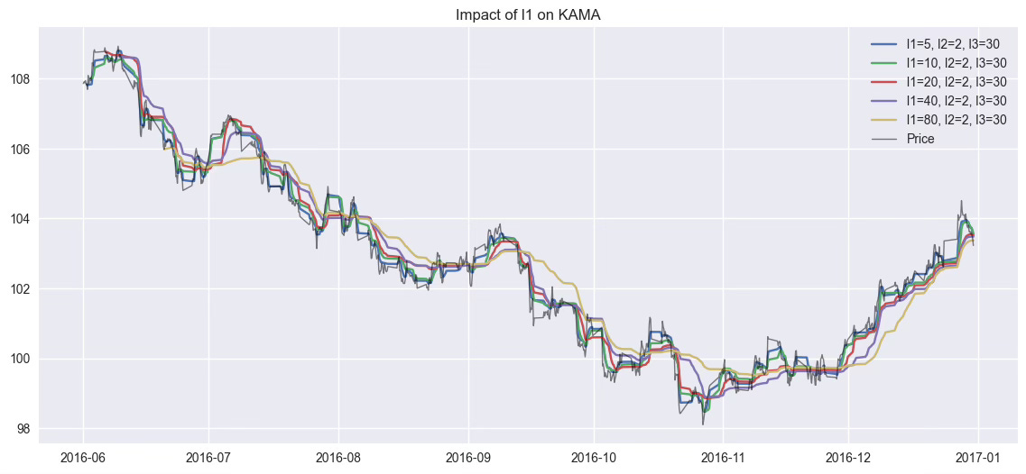
l1 defines how far back the KAMA looks to assess price efficiency. Smaller values make the KAMA more reactive but sensitive to noise.
Larger values smooth it out, but increase lag.
Trade-off: reactivity vs. stability.

👉 This is the main slider between noise and responsiveness.

4.2. Effect of l2 (Fast Period)

To explore how l2 affects the reactivity of KAMA, we fix l1=10 and l3=30, and vary l2 across [1, 2, 3, 5, 10].

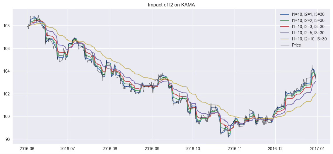
l2 controls the maximum reactivity of KAMA when the market is clean (ER ≈ 1). Lower values make KAMA more agile in trends.
Higher values slow down reactions, even in trending conditions.
It sets the upper speed limit of the moving average.

👉 l2 controls KAMA's maximum reaction speed.

4.3. Effect of `l3` (Slow Period)

To examine how l3 influences KAMA’s behavior in noisy markets, we fix l1=10 and l2=2, and vary l3 across [10, 20, 30, 60, 100].

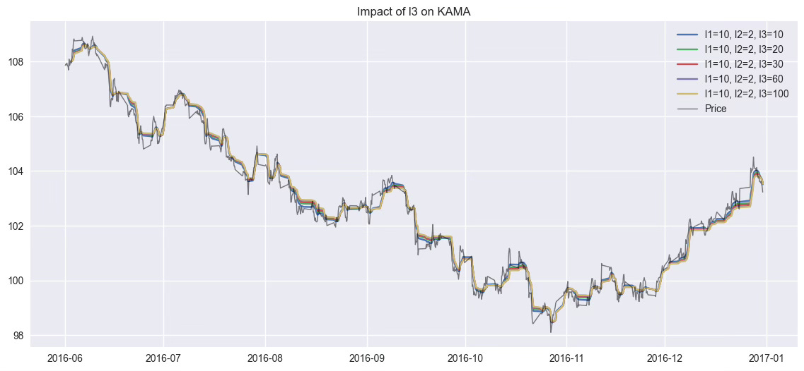
l3 sets the minimum reactivity of KAMA in noisy or sideways markets (ER ≈ 0). Smaller values let KAMA move even in choppy markets. Larger values freeze it when there's no clear trend.
It acts like a safety brake during uncertainty.

👉 l3 acts as an “emergency brake” in range phases.

⚡ You can use the optimized kama() function directly from the Quantreo library, no need to rebuild it yourself.

💻 Find the code of this post here

KAMA isn’t just another moving average. It’s a smart, adaptive tool that adjusts its sensitivity based on market behavior.
But to truly benefit from it, you need to understand how it works, not just how to call the function.

In this guide, we covered:

The intuition and math behind KAMA
A clean, step-by-step implementation
A visual breakdown of how each parameter impacts the curve

Whether you're building signals, filtering noise, or designing adaptive strategies, KAMA gives you fine control, as long as you know how to tune it.