

Kalman Filter in Trading (1/2)
A simple mental model to blend predictions and noisy observations

In trading, almost everything you touch is noisy. Prices jump because of microstructure, spreads widen for a few prints, volatility spikes just because your window is short. If you react to every wiggle, you trade randomness. If you smooth too much, you react too late.
The Kalman filter is a clean way to sit in the middle. It estimates a “true signal” behind noisy observations by doing the same two-step loop every time: predict what should happen, then correct using what you observed. The correction is not arbitrary. It is weighted by uncertainty, which is why Kalman feels both smooth and responsive.
1) The problem, in one minute
Markets are messy. Your indicators are messier.
A price series mixes real moves with microstructure noise. A rolling volatility mixes real regime shifts with estimation error.
Same story for any feature built on finite windows. Feed that raw signal into a strategy and you get false triggers, unstable sizing, and lots of noise masquerading as information.
What we want is simple. Keep the information, drop the useless wiggles.
2) The key idea. Two realities
Kalman starts with a clean separation.
What you observe: y_t (noisy)
What you want: x_t (latent state, hidden signal)
You assume:
where v_t is measurement noise.
The “latent state” is not a mystical fair value. It is simply the signal you choose to model: a smoother price level, a latent volatility, a stable trend component, a cleaner spread.
A tiny example (with a simulated “latent signal”)
To make this concrete, we can build a toy signal.
First, we create a latent state x_t. Think of it as the clean underlying level we wish we could observe.
Then we generate what the market actually shows us:
\(y_t=x_t+noise\)This mimics noisy prints, bid ask bounce, and random micro wiggles.
In a simulation, we can plot both x_t and y_t. This lets us visually check whether the Kalman estimate is actually recovering the hidden signal.
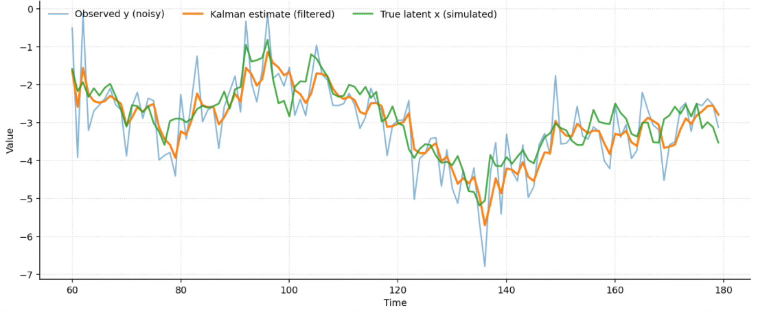
Important: In real trading, we never see x_t. That is the whole point. The filter is valuable precisely because it produces an estimation of x_t, a disciplined estimate of what might be behind y_t.
We do not trade y. We trade an estimate of what is behind y.
3) Kalman is a two-step loop
Kalman is a loop with one question repeated forever:
What did I expect? What did I see? How much should I adjust?
Predict
You start each step with a belief about the hidden signal. Then you move it forward using a simple model.
This is your prior. It is what you believe before seeing the new data point.
t∣t−1 means: estimate at time t using information up to t−1 (before seeing y_t)
My best guess for the hidden level today is yesterday’s filtered estimate.
Update
Then you look at the new observation and measure the surprise:
Finally you adjust toward the observation:
The updated estimate is always “between” the prediction and the observation. The only thing that decides where you land is the gain K_t.
K_t is the trust weight you give to the new observation.
K_t≈1 means “I trust the data”. Fast reaction, little smoothing.
K_t≈0 means “I trust the model”. Slow reaction, strong smoothing.
4) Focus on the Kalman Gain K_t
The gain K_t is the adaptive weight that controls the update. It answers one question:
Do I trust the new observation, or do I trust my current belief?
In the simplest 1D case, the gain is computed from two sources of uncertainty:
Prediction uncertainty (how unsure you are before seeing the new point)
Measurement noise (how noisy the observation is)
Here are the two key equations.
Each step forward adds uncertainty. Q is how much you allow the hidden signal to “wander” between two observations. Bigger Q means “the state can move fast”, so you become more willing to adjust.
The gain compares how uncertain your prediction is versus how noisy the observation is.
Bigger R means noisier data. The gain shrinks. You smooth more.
Bigger Q makes your prediction less certain (through P). The gain grows. You adapt faster.
So the only real knobs you set in practice are Q and R:
R controls how much you distrust the data.
Q controls how flexible the hidden signal is.
In the next newsletter, we will walk through a simple trading example and show how to use the Kalman estimate in a real signal.
Yes, there were a few equations here, but the goal is not to memorize them. The goal is to internalize the intuition: predict, measure the surprise, and adjust by an uncertainty weighted amount.
👉 If you want to go deeper into each step of the strategy building process, with real-life projects, ready-to-use templates, and 1:1 mentoring, that’s exactly what the Alpha Quant Program is for.