Building a Clean Research Environment with Oryon

How to combine features and targets in one dataframe before doing exploratory data analysis.

Exploratory data analysis in quant often becomes messy much faster than expected.

Features are computed in one place, targets in another, and then everything has to be aligned manually before any real analysis can begin. That usually means extra joins, shifting logic, duplicated code, and a higher risk of silent mistakes.

The issue is not computing features or targets. The issue is creating a research dataset where both live together cleanly and can be analyzed immediately.

---

1. The Oryon Approach

With Oryon, the process stays simple. You build a FeaturePipeline, a TargetPipeline, run both on the same market data, and join the outputs into a single dataframe.

from oryon.datasets import load_sample_bars
from oryon import FeaturePipeline
from oryon.features import Sma, ParkinsonVolatility, Correlation, ShannonEntropy, Adf
from oryon.scalers import RollingZScore
from oryon.adapters import run_features_pipeline_pandas


# Import sample data (OHLCV bars)
df = load_sample_bars()

# Create the features list
features_list = [
    Correlation(inputs=["close", "volume"], window=30, outputs=["close_volume_corr_30"]),
    ParkinsonVolatility(inputs=["high","low"], window=50, outputs=["close_pvol_50"]),
    Adf(inputs=["close"], window=100, outputs=["close_adf_100", "close_adf_pval_100"])
]

# Create the scalers list to apply z-score to all the wanted features
scalers_list = [RollingZScore(inputs=[col], window=2000, outputs=[f"z_{col}"]) for col in [
    "close_volume_corr_30", "close_pvol_50", "close_adf_pval_100"
]]

# Combine both list
features_list.extend(scalers_list)

# Create the pipeline object (that can run to on live trading)
pipe = FeaturePipeline(features_list, input_columns=["close", "high", "low", "volume"])

# Run the pipeline on the sample data
df_features = run_features_pipeline_pandas(pipe, df)

from oryon import TargetPipeline
from oryon.adapters import run_targets_pipeline_pandas
from oryon.targets import FutureReturn, FutureLinearSlope

# Essential for the FutureLinearSlope (x=time, y=price)
df["constant_time"] = [i for i in range(len(df))] # Essential for the FutureLinearSlope (x=time, y=price)

# Create the targets list
targets_list = [
    FutureLinearSlope(inputs=["constant_time", "close"], horizon=20, outputs=["future_slope_20", "r2_future_slope_20"]),
    FutureLinearSlope(inputs=["constant_time", "close"], horizon=50, outputs=["future_slope_50", "r2_future_slope_50"]),
    FutureReturn(inputs=["close"], horizon=10, outputs=["future_returns_2"])
]

# Create the target pipeline object
target_pipe = TargetPipeline(targets_list, input_columns=["constant_time", "close"])

# Run the pipeline
df_targets = run_targets_pipeline_pandas(target_pipe, df)

# Ready-to-use dataframe
df_research = df_features.join(df_targets)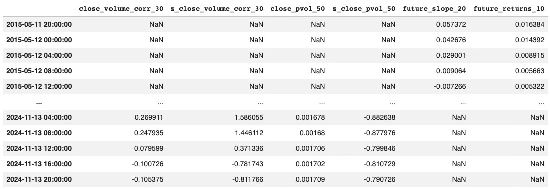

The result is a single research table where engineered features and forward-looking targets are already aligned and ready to explore.

---

3. Why This Matters

Once everything is in the same dataframe, EDA becomes much easier.

You can immediately start testing simple relationships between inputs and outputs, whether through correlation, mutual information, or more advanced selection methods. Instead of spending time preparing the dataset, you can focus on extracting useful structure from it.

That is the real value of a clean research environment: less plumbing, more analysis.

If you want to take this further and connect feature pipelines with AI agents, you can take a look at AI Trading Lab.

Oryon is now available in beta.

If you want to take a closer look at the library and its design, you can explore it directly on GitHub.

And if you find it useful, consider adding a star. it helps more than it seems.